These symptoms are often blamed on the luminaire. In practice, the cause may be the distribution circuit: too much current on a long cable, an undersized conductor, cumulative resistance at outdoor joints, or a power supply placed for convenience rather than electrical performance.
Low-voltage systems make the arithmetic especially important. A loss of 1.2V is only about 0.5% of a 230V supply, but it is 5% of a 24V supply. The same cable resistance therefore has a much larger effect on the available voltage at a 24V luminaire.
This guide shows how to estimate voltage drop, compare cable sizes, calculate a branch with distributed luminaires and decide when moving or splitting the power supply is more effective than adding copper. It is written for 24V DC constant-voltage outdoor luminaires designed to accept a 24V supply. It is not a method for driving a bare LED board directly.

Important: This article provides a calculation and procurement framework, not an approved wiring design. Cable selection must also satisfy current-carrying capacity, fault protection, insulation, environmental, burial, connector and local electrical-code requirements. Final design and installation should be completed by qualified professionals.
Quick Answer
- Start with the exact 24V luminaire input power or current, quantity and control condition—not only the LED chip wattage.
- Record cable length as the one-way route length. A two-wire DC circuit includes both outgoing and return conductors.
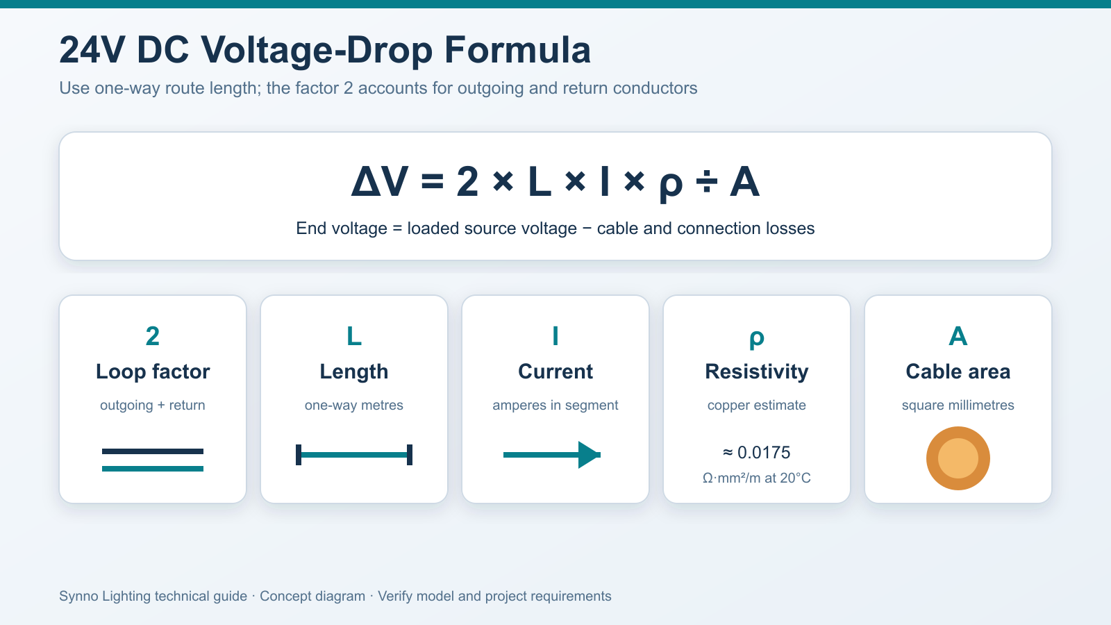
- For a preliminary copper-cable estimate, use ΔV = 2 × L × I × ρ ÷ A. Here, L is one-way length, I is circuit current, ρ is conductor resistivity and A is conductor area.
- Calculate end voltage = loaded power-supply terminal voltage − cable and connection losses. Confirm that it stays within the exact luminaire's permitted input range and the project's brightness-consistency target.
- For luminaires spaced along a branch, calculate each segment separately because current decreases after every take-off.
- A larger cable can reduce drop, but shorter runs, additional zones or a more central power-supply location may be more economical and maintainable.
- Do not apply a universal “3%,” “5%” or “80% loading” rule without checking the applicable electrical standard, luminaire data, power-supply instructions and project criteria.
1. Define the 24V System Before Choosing a Cable
The phrase “24V landscape lighting” is not a complete electrical specification. Before any calculation, confirm the system boundary.
This article assumes:
- a regulated 24V DC constant-voltage power supply;
- complete outdoor luminaires designed for 24V DC input;
- a two-conductor distribution circuit;
- copper conductors;
- luminaires connected in parallel, not in series;
- steady-state maximum operating load as the first calculation condition.
The real project may add PWM dimming, RGB/RGBW controllers, addressable control, long control cables, emergency functions or multiple output channels. Those interfaces can change conductor count, current per core, switching behaviour and commissioning requirements.
Do not use this method to select the current for a bare LED module. A complete 24V luminaire may contain its own regulation, polarity protection or control electronics. The relevant input current and acceptable voltage range must come from the exact luminaire configuration.
Also, 24V does not automatically mean SELV. The safety classification depends on the source, isolation, circuit arrangement and applicable installation requirements. Ask for the power supply's safety information and have the complete circuit classified by the project electrical designer.
2. Why a Small Resistance Matters at 24V
Every conductor and joint has resistance. When current flows, that resistance produces a voltage difference:
Voltage drop = current × resistance
It also produces heat:
Power loss = current² × resistance
This creates two practical effects. First, higher branch current increases voltage drop. Second, the heating loss rises with the square of current. Combining many luminaires onto one long branch can therefore be much less efficient than dividing the same total load between shorter branches.
The percentage also changes with system voltage. Consider the same 1V loss:
| Nominal supply | 1V loss as a percentage |
|---|---|
| 230V | 0.43% |
| 48V | 2.08% |
| 24V | 4.17% |
| 12V | 8.33% |
This is one reason 24V systems are often preferred to 12V for longer low-voltage distribution. Synno's article on 12V and 24V pool-lighting safety introduces that comparison. The present guide goes further by showing how to calculate the circuit rather than relying on the voltage label alone.
3. The Inputs Required for a Useful Calculation
Prepare a simple branch schedule before opening a calculator.
| Required input | Why it matters |
|---|---|
| Exact luminaire model and configuration | Wattage, input range and electronics can vary within one housing family |
| Quantity on each branch | Determines total steady-state load |
| Input watts or current per luminaire | Defines branch current; use luminaire input data, not nominal LED-chip watts |
| One-way cable length | The formula accounts separately for outgoing and return conductors |
| Fixture positions along the route | Required for segment-by-segment calculation |
| Cable material and conductor area | Determines conductor resistance |
| Conductor temperature or manufacturer resistance data | Copper resistance rises as temperature increases |
| Loaded power-supply output voltage | Nominal “24V” may not equal the measured voltage at full load |
| Luminaire permitted input-voltage range | Sets the electrical limit at the far end |
| Project uniformity target | A luminaire may remain on but still fail the required visual consistency |
| Control and start-up condition | Dimming controllers and inrush can create additional constraints |
| Joint and connector count | Outdoor connections add resistance and potential failure points |
The best source for conductor resistance is the selected cable manufacturer's data at the relevant temperature. A resistivity value is useful for early comparison, but it does not replace the final cable datasheet.
4. The Basic 24V DC Voltage-Drop Formula
For a two-wire copper circuit with the load treated at the end of the branch:
ΔV = 2 × L × I × ρ ÷ A
Where:
- ΔV = voltage drop in volts;
- L = one-way cable length in metres;
- I = branch current in amperes;
- ρ = conductor resistivity in Ω·mm²/m;
- A = conductor cross-sectional area in mm²;
- 2 = outgoing plus return path.
For an early estimate, copper resistivity is often represented as approximately 0.0175 Ω·mm²/m at 20°C. This is an illustrative calculation value, not a cable compliance value. Actual conductor resistance depends on construction and temperature.
Then calculate:
Voltage-drop percentage = ΔV ÷ 24V × 100%
Estimated end voltage = loaded source voltage − ΔV
If the cable datasheet gives resistance in Ω/km, the more direct method is:
ΔV = I × Rloop
where Rloop includes both outgoing and return conductor resistance for the actual length and temperature.
The installation framework also matters. IEC 60364-5-52 addresses selection and erection of wiring systems and includes voltage-drop considerations. The applicable limit and calculation method must be established under the project’s adopted standard and national rules; a blog percentage should not be treated as a universal legal limit.
5. Worked Example: Eight 6W Luminaires on a 30m Branch
Assume the following preliminary design:
- eight 24V luminaires;
- 6W input per luminaire at the design condition;
- 48W total input;
- 30m one-way route;
- 2.5mm² copper conductors;
- all load treated at the cable end for a conservative first estimate;
- 24.0V measured at the power-supply output under load.
Step 1: Estimate branch current
I = P ÷ V = 48W ÷ 24V = 2.0A
This is a preliminary steady-state value. Confirm the actual input current and start-up behaviour from the exact luminaire and controller data.
Step 2: Estimate cable voltage drop
ΔV = 2 × 30m × 2.0A × 0.0175 ÷ 2.5mm² = 0.84V
Step 3: Convert to a percentage
0.84V ÷ 24V × 100% = 3.5%
Step 4: Estimate voltage at the remote load
24.0V − 0.84V = 23.16V
The calculation does not finish with “3.5% is acceptable.” The next questions are:
- Is 23.16V within the exact luminaire's declared input range under all operating conditions?
- Does the luminaire maintain the required output and control stability at that voltage?
- What additional loss is expected in fuses, controllers, terminals and outdoor connectors?
- What is the cable resistance at the expected operating temperature?
- Does the cable satisfy current-carrying capacity and protective-device requirements?
The acceptable design drop should come from those answers.
6. Cable-Size Comparison for the Same Example
Keeping the 2A load and 30m one-way length unchanged illustrates the value of conductor area.
| Copper conductor area | Estimated drop | Drop at 24V | Estimated end voltage |
|---|---|---|---|
| 1.5mm² | 1.40V | 5.83% | 22.60V |
| 2.5mm² | 0.84V | 3.50% | 23.16V |
| 4.0mm² | 0.53V | 2.19% | 23.48V |
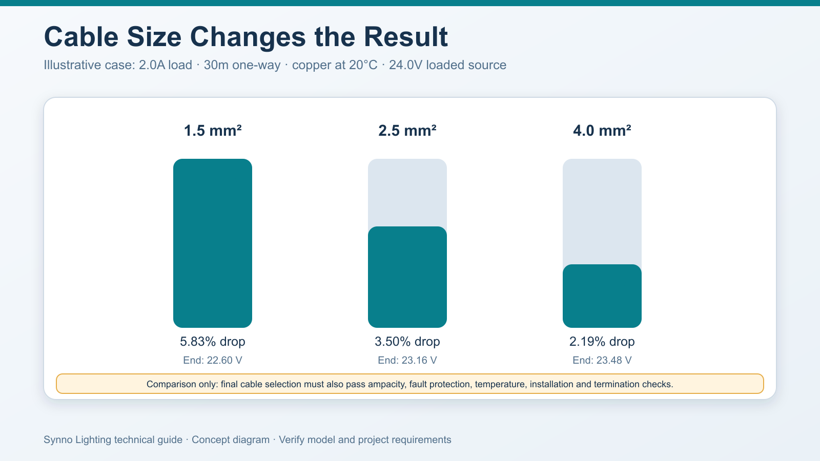
The table is not a universal cable-size chart. If current or length changes, the result changes. A 4mm² conductor can still be inadequate on a longer or more heavily loaded branch, while 1.5mm² may be electrically adequate for a short, lightly loaded branch if all other requirements are met.
Cost must also include terminals and glands. A larger conductor may not fit the luminaire's supplied cable, connector or junction box. The transition detail must be specified rather than forced on site.
7. Distributed Loads Must Be Calculated Segment by Segment
The previous example treats all eight luminaires as if they were at the end of the 30m cable. That is a useful conservative screening method, but it overstates cable drop when luminaires are distributed along the route.
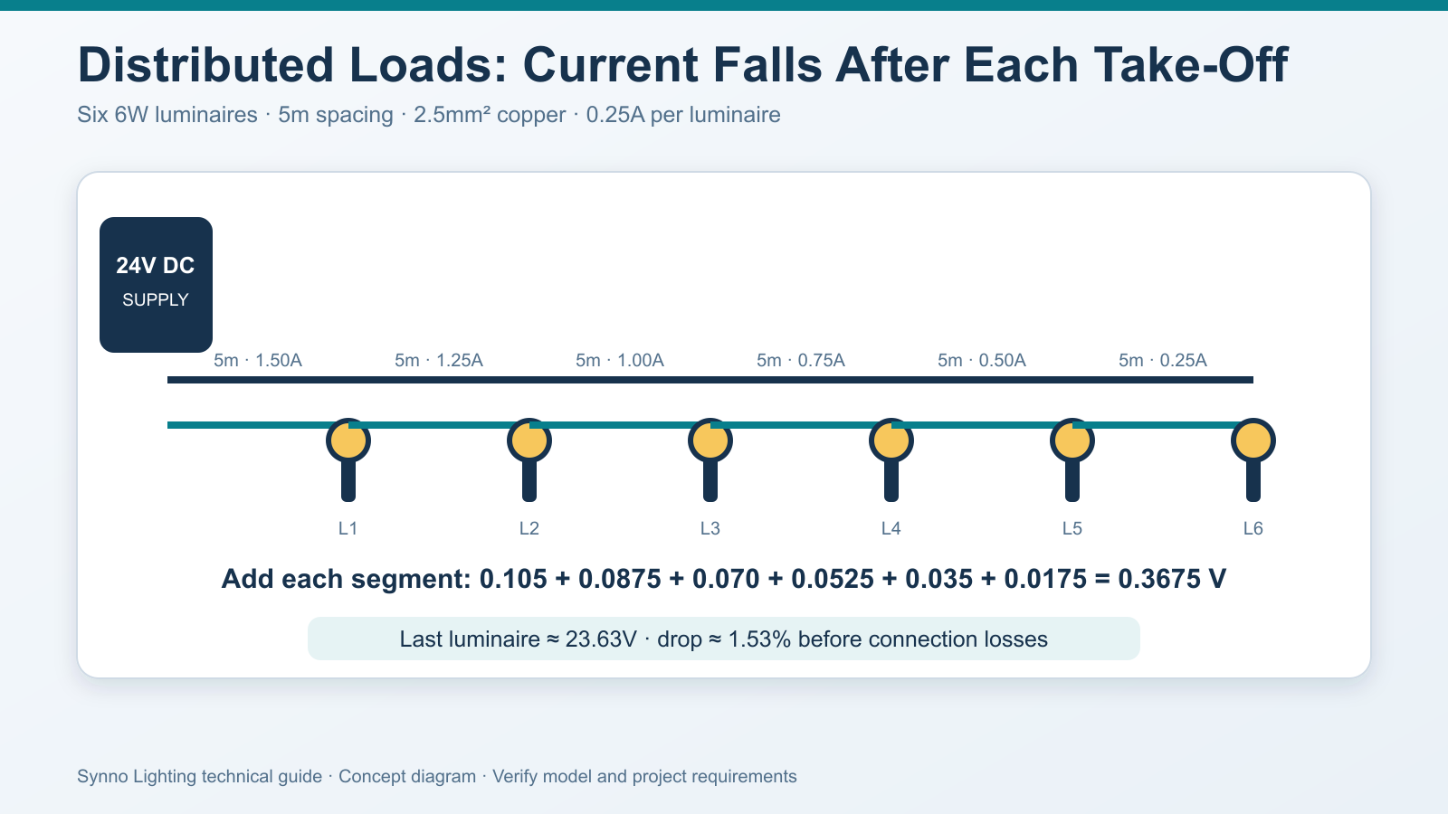
Consider six 6W luminaires, each 5m apart, supplied at 24V through 2.5mm² copper conductors. Each luminaire draws approximately:
6W ÷ 24V = 0.25A
The first cable segment carries all six luminaires, or 1.50A. After the first take-off, the next segment carries 1.25A. Current continues to reduce toward the end.
| 5m segment | Load remaining downstream | Segment current | Segment drop |
|---|---|---|---|
| 1 | 6 luminaires | 1.50A | 0.105V |
| 2 | 5 luminaires | 1.25A | 0.0875V |
| 3 | 4 luminaires | 1.00A | 0.070V |
| 4 | 3 luminaires | 0.75A | 0.0525V |
| 5 | 2 luminaires | 0.50A | 0.035V |
| 6 | 1 luminaire | 0.25A | 0.0175V |
| Total to last luminaire | — | — | 0.3675V |
The estimated last-luminaire voltage is therefore:
24.0V − 0.3675V = 23.6325V
The drop is approximately 1.53%, before adding connection and device losses.
Two common shortcuts cause mistakes:
- Applying the full branch current to the entire route can be unnecessarily conservative for a distributed load.
- Applying only the last luminaire's current to the entire route can seriously underestimate drop.
A spreadsheet with one row per cable segment is usually the clearest project record.
8. Compare the Main Distribution Topologies
Home-run or star circuits
Each branch returns directly to the power-supply or zone cabinet. Voltage-drop calculations are predictable and one branch fault affects fewer luminaires. The trade-off is more cable, terminals and protective devices.
Radial or daisy-chain circuit
One trunk passes each luminaire in sequence. It may use less cable, but voltage drop accumulates and the first segments carry the highest current. Joint quality and segment calculations become critical.
Trunk with short branches
A suitably sized trunk supplies several short local branches. This can balance copper use, voltage performance and access for maintenance, but branch protection and junction details must be designed clearly.
Do not improvise a ring feed
Feeding a branch from both ends may appear to solve voltage drop, but current sharing, conductor polarity, fault isolation and protection coordination become more complex. Do not create a parallel or ring arrangement unless it is specifically engineered and documented.
9. Power-Supply Location Can Save More Copper Than Upsizing Every Cable
If one central cabinet sits at the edge of a large garden, every remote branch may be long. Moving the source closer to the electrical centre of the loads reduces cable length. Splitting one large zone into two or more accessible supply zones can also reduce both branch length and branch current.
The IEC's energy-efficiency guidance for electrical installations describes reducing conductor length by locating supply points near the barycentre of loads and reducing losses through appropriate conductor sizing. The idea is simple: distribution layout is part of energy performance, not just a drafting decision.
Compare three concepts:
- One distant central source: simple maintenance point, but long high-current DC branches.
- One centrally located source: shorter average branch length, if a safe accessible location exists.
- Several zone sources: shorter lower-current branches and easier fault isolation, balanced against more enclosures, AC feeds and maintenance points.
A real large-site example comes from Signify's published Meryal Water Park project, where a 24V DC outdoor lighting system used multiple feeder-pillar locations and the team redesigned load schedules and cable sizes after voltage-drop calculations. The lesson is not to copy a project count; it is to coordinate equipment location, load schedule and cable design early.
Power supplies and junctions must remain accessible and suitable for their environment. Do not hide them in soil, permanently seal them behind finishes, or place them where irrigation and drainage create avoidable exposure.
10. Size the Power Supply from Verified Input Data
Add the input power of every luminaire and controller on the output, then account for the manufacturer's loading, ambient-temperature and derating instructions.
Preliminary connected load = quantity × actual input watts per luminaire + controller/accessory loads
Do not automatically apply a universal “use only 80% of the power supply” rule. Some products and jurisdictions have continuous-load provisions, while power-supply derating curves may depend on input voltage, ambient temperature, orientation and enclosure ventilation. Use the selected power supply's manual and the project electrical rules.
Also check:
- output-current limit and overload behaviour;
- start-up and inrush behaviour of all connected luminaires and controllers;
- short-circuit and branch protection;
- operating temperature inside the enclosure;
- cable loss and connection loss;
- compatibility with dimming or PWM controllers;
- maximum output-cable length or capacitance restrictions in the manual;
- EMC and safety requirements for the complete installation.
Manufacturer limits can be very specific. For example, one Tridonic 24V constant-voltage driver datasheet limits the secondary cable to 2m, while another archived model describes a cable-length limit based on 1V drop. These are product-specific instructions, not universal 24V limits. They show why the selected power-supply manual must be part of the design file.
11. Why Raising the Output Voltage Is Not a General Fix
Some installers try to compensate for a weak last luminaire by turning an adjustable power supply above 24V. This can create three problems:
- luminaires near the source receive the highest voltage and may exceed their permitted input;
- the adjustment may invalidate the approved configuration or reduce component life;
- voltage still changes with load, temperature and connection condition.
Only adjust a power supply within its documented range and as part of an engineered design that verifies the voltage at every connected luminaire. If the supply includes remote-sense terminals, follow its manual exactly. Remote sense has model-specific compensation limits and wiring requirements; it is not permission to ignore cable size.
MEAN WELL's official LED power-supply guidance likewise notes that extending DC cable requires line-drop consideration because excessive drop can prevent the LED load from operating correctly. The robust solution is usually to reduce resistance, reduce current per branch, shorten the route or relocate the source.
12. Outdoor Joints Can Undo a Good Cable Calculation
The formula assumes known conductor resistance. Real outdoor circuits add terminals, connectors, fuses, controller outputs and splices.
A dry, correctly crimped connection may add little loss. A loose terminal, undersized connector or water-contaminated splice can add enough resistance to create local heating and intermittent voltage. The problem may appear only after thermal cycling or rain.
Specify:
- compatible cable outside diameter and gland clamping range;
- conductor material, strand preparation and terminal type;
- connector current, voltage and environmental rating;
- branch-box ingress protection and drainage position;
- strain relief and pull-out resistance;
- polarity identification;
- accessible joint locations for testing;
- approved method for transitions between trunk cable and luminaire leads.
IP rating does not describe every installation detail. A high-IP luminaire connected through a poor field joint can still become an unreliable system.
13. Cable Size Must Pass More Than the Voltage-Drop Check
A conductor that produces an acceptable drop can still be unsuitable. Final selection should verify at least:
- current-carrying capacity under the actual installation method;
- ambient and soil temperature;
- grouping and thermal insulation effects;
- short-circuit withstand and protective-device operation;
- insulation voltage and compatibility with the circuit classification;
- UV, moisture, chemical and mechanical resistance;
- burial depth, conduit fill and pulling requirements;
- connector, gland and terminal capacity;
- national rules for outdoor and underground wiring;
- voltage drop under the project design condition.
For buried or ground-mounted products, installation quality remains as important as the electrical calculation. Synno's underground LED light installation guide explains drainage, sleeves and cable-routing considerations for inground applications.
14. Commission the Circuit Under Load
Do not approve the branch from an open-circuit reading alone. A 24.0V measurement with the luminaires disconnected says little about loaded voltage drop.
Use a documented commissioning sequence:
- Verify the circuit, polarity, protection and isolation before energizing.
- Measure the power-supply output voltage with the designed load operating.
- Measure voltage at the first and last luminaire, and at any critical branch point.
- Record steady-state branch current at the maximum intended operating condition.
- Test the control scene that produces the greatest simultaneous load.
- Check for visible output differences, flicker, resets or control instability.
- Inspect accessible joints for abnormal voltage difference or temperature rise using approved procedures.
- Compare readings with the exact luminaire input range and design target.
- Save the results with the as-built cable lengths, conductor sizes and joint locations.
Measure at the luminaire input or defined test point—not at an unrelated cabinet terminal. Use touch-safe methods and qualified personnel appropriate to the installation.
15. A Practical Design Workflow
Step 1: Build a model-specific load schedule
List every luminaire, controller and accessory by order code. Do not mix samples with production substitutions.